3.1 HTML document
As we just mentioned before, Markdown was originally designed for HTML output, so it may not be surprising that the HTML format has the richest features among all output formats. We recommend that you read this full section before you learn other output formats, because other formats have several features in common with the HTML document format, and we will not repeat these features in the corresponding sections.
To create an HTML document from R Markdown, you specify the html_document output format in the YAML metadata of your document:
---
title: Habits
author: John Doe
date: March 22, 2005
output: html_document
---
3.1.1 Table of contents
You can add a table of contents (TOC) using the toc option and specify the depth of headers that it applies to using the toc_depth option. For example:
---
title: "Habits"
output:
  html_document:
    toc: true
    toc_depth: 2
---
If the table of contents depth is not explicitly specified, it defaults to 3 (meaning that all level 1, 2, and 3 headers will be included in the table of contents).
3.1.1.1 Floating TOC
You can specify the toc_float option to float the table of contents to the left of the main document content. The floating table of contents will always be visible even when the document is scrolled. For example:
---
title: "Habits"
output:
  html_document:
    toc: true
    toc_float: true
---
You may optionally specify a list of options for the toc_float parameter which control its behavior. These options include:
collapsed(defaults toTRUE) controls whether the TOC appears with only the top-level (e.g., H2) headers. If collapsed initially, the TOC is automatically expanded inline when necessary.smooth_scroll(defaults toTRUE) controls whether page scrolls are animated when TOC items are navigated to via mouse clicks.
For example:
---
title: "Habits"
output:
  html_document:
    toc: true
    toc_float:
      collapsed: false
      smooth_scroll: false
---
3.1.2 Section numbering
You can add section numbering to headers using the number_sections option:
---
title: "Habits"
output:
  html_document:
    toc: true
    number_sections: true
---
Note that if you do choose to use the number_sections option, you will likely also want to use # (H1) headers in your document as ## (H2) headers will include a decimal point, because without H1 headers, you H2 headers will be numbered with 0.1, 0.2, and so on.
3.1.3 Tabbed sections
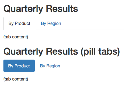
You can organize content using tabs by applying the .tabset class attribute to headers within a document. This will cause all sub-headers of the header with the .tabset attribute to appear within tabs rather than as standalone sections. For example:
## Quarterly Results {.tabset}

### By Product

(tab content)

### By Region

(tab content)
You can also specify two additional attributes to control the appearance and behavior of the tabs. The .tabset-fade attribute causes the tabs to fade in and out when switching between tabs. The .tabset-pills attribute causes the visual appearance of the tabs to be “pill” (see Figure 3.1) rather than traditional tabs. For example:
## Quarterly Results {.tabset .tabset-fade .tabset-pills}
FIGURE 3.1: Traditional tabs and pill tabs on an HTML page.
3.1.4 Appearance and style
There are several options that control the appearance of HTML documents:
themespecifies the Bootstrap theme to use for the page (themes are drawn from the Bootswatch theme library). Valid themes include default, cerulean, journal, flatly, darkly, readable, spacelab, united, cosmo, lumen, paper, sandstone, simplex, and yeti. Passnullfor no theme (in this case you can use thecssparameter to add your own styles).highlightspecifies the syntax highlighting style. Supported styles includedefault,tango,pygments,kate,monochrome,espresso,zenburn,haddock,breezedark, andtextmate. Passnullto prevent syntax highlighting.smartindicates whether to produce typographically correct output, converting straight quotes to curly quotes,---to em-dashes,--to en-dashes, and...to ellipses. Note thatsmartis enabled by default.
For example:
---
title: "Habits"
output:
  html_document:
    theme: united
    highlight: tango
---
3.1.4.1 Custom CSS
You can add your own CSS to an HTML document using the css option:
---
title: "Habits"
output:
  html_document:
    css: styles.css
---
If you want to provide all of the styles for the document from your own CSS you set the theme (and potentially highlight) to null:
---
title: "Habits"
output:
  html_document:
    theme: null
    highlight: null
    css: styles.css
---
You can also target specific sections of documents with custom CSS by adding ids or classes to section headers within your document. For example the following section header:
## Next Steps {#nextsteps .emphasized}Would enable you to apply CSS to all of its content using either of the following CSS selectors:
#nextsteps {
   color: blue;
}

.emphasized {
   font-size: 1.2em;
}
3.1.5 Figure options
There are a number of options that affect the output of figures within HTML documents:
fig_widthandfig_heightcan be used to control the default figure width and height (7x5 is used by default).fig_retinaspecifies the scaling to perform for retina displays (defaults to 2, which currently works for all widely used retina displays). Set tonullto prevent retina scaling.fig_captioncontrols whether figures are rendered with captions.devcontrols the graphics device used to render figures (defaults topng).
For example:
---
title: "Habits"
output:
  html_document:
    fig_width: 7
    fig_height: 6
    fig_caption: true
---
3.1.6 Data frame printing
You can enhance the default display of data frames via the df_print option. Valid values are shown in Table 3.1.
| Option | Description |
|---|---|
| default | Call the print.data.frame generic method |
| kable | Use the knitr::kable function |
| tibble | Use the tibble::print.tbl_df function |
| paged | Use rmarkdown::paged_table to create a pageable table |
3.1.6.1 Paged printing
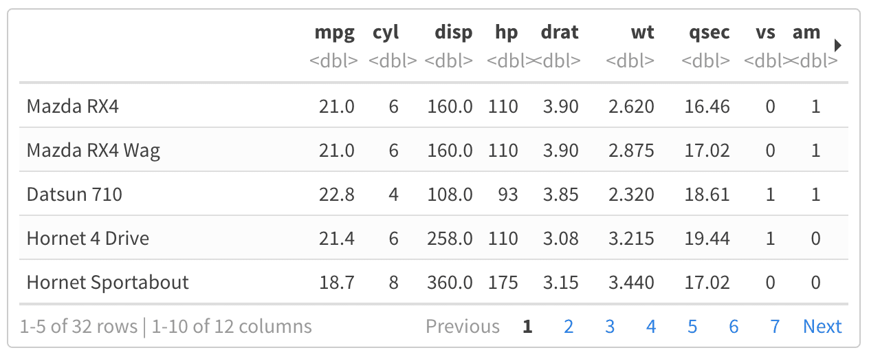
When the df_print option is set to paged, tables are printed as HTML tables with support for pagination over rows and columns. For instance (see Figure 3.2):
---
title: "Motor Trend Car Road Tests"
output:
  html_document:
    df_print: paged
---

```{r}
mtcars
```
FIGURE 3.2: A paged table in the HTML output document.
Table 3.2 shows the available options for paged tables.
| Option | Description |
|---|---|
| max.print | The number of rows to print. |
| rows.print | The number of rows to display. |
| cols.print | The number of columns to display. |
| cols.min.print | The minimum number of columns to display. |
| pages.print | The number of pages to display under page navigation. |
| paged.print | When set to FALSE turns off paged tables. |
| rownames.print | When set to FALSE turns off row names. |
These options are specified in each chunk like below:
```{r cols.print=3, rows.print=3}
mtcars
```
3.1.7 Code folding
When the knitr chunk option echo = TRUE is specified (the default behavior), the R source code within chunks is included within the rendered document. In some cases, it may be appropriate to exclude code entirely (echo = FALSE) but in other cases you might want the code to be available but not visible by default.
The code_folding: hide option enables you to include R code but have it hidden by default. Users can then choose to show hidden R code chunks either individually or document wide. For example:
---
title: "Habits"
output:
  html_document:
    code_folding: hide
---
You can specify code_folding: show to still show all R code by default but then allow users to hide the code if they wish.
3.1.8 MathJax equations
By default, MathJax scripts are included in HTML documents for rendering LaTeX and MathML equations. You can use the mathjax option to control how MathJax is included:
Specify
"default"to use an HTTPS URL from a CDN host (currently provided by RStudio).Specify
"local"to use a local version of MathJax (which is copied into the output directory). Note that when using"local"you also need to set theself_containedoption tofalse.Specify an alternate URL to load MathJax from another location.
Specify
nullto exclude MathJax entirely.
For example, to use a local copy of MathJax:
---
title: "Habits"
output:
  html_document:
    mathjax: local
    self_contained: false
---
To use a self-hosted copy of MathJax:
---
title: "Habits"
output:
  html_document:
    mathjax: "http://example.com/MathJax.js"
---
To exclude MathJax entirely:
---
title: "Habits"
output:
  html_document:
    mathjax: null
---
3.1.9 Document dependencies
By default, R Markdown produces standalone HTML files with no external dependencies, using data: URIs to incorporate the contents of linked scripts, stylesheets, images, and videos. This means you can share or publish the file just like you share Office documents or PDFs. If you would rather keep dependencies in external files, you can specify self_contained: false. For example:
---
title: "Habits"
output:
  html_document:
    self_contained: false
---
Note that even for self-contained documents, MathJax is still loaded externally (this is necessary because of its big size). If you want to serve MathJax locally, you should specify mathjax: local and self_contained: false.
One common reason to keep dependencies external is for serving R Markdown documents from a website (external dependencies can be cached separately by browsers, leading to faster page load times). In the case of serving multiple R Markdown documents you may also want to consolidate dependent library files (e.g. Bootstrap, and MathJax, etc.) into a single directory shared by multiple documents. You can use the lib_dir option to do this. For example:
---
title: "Habits"
output:
  html_document:
    self_contained: false
    lib_dir: libs
---
3.1.10 Advanced customization
3.1.10.1 Keeping Markdown
When knitr processes an R Markdown input file, it creates a Markdown (*.md) file that is subsequently transformed into HTML by Pandoc. If you want to keep a copy of the Markdown file after rendering, you can do so using the keep_md option:
---
title: "Habits"
output:
  html_document:
    keep_md: true
---
3.1.10.2 Includes
You can do more advanced customization of output by including additional HTML content or by replacing the core Pandoc template entirely. To include content in the document header or before/after the document body, you use the includes option as follows:
---
title: "Habits"
output:
  html_document:
    includes:
      in_header: header.html
      before_body: doc_prefix.html
      after_body: doc_suffix.html
---
3.1.10.3 Custom templates
You can also replace the underlying Pandoc template using the template option:
---
title: "Habits"
output:
  html_document:
    template: quarterly_report.html
---
Consult the documentation on Pandoc templates for additional details on templates. You can also study the default HTML template default.html5 as an example.
3.1.10.4 Markdown extensions
By default, R Markdown is defined as all Pandoc Markdown extensions with the following tweaks for backward compatibility with the old markdown package (Allaire et al. 2019):
+autolink_bare_uris
+tex_math_single_backslash
You can enable or disable Markdown extensions using the md_extensions option (you preface an option with - to disable and + to enable it). For example:
---
title: "Habits"
output:
  html_document:
    md_extensions: -autolink_bare_uris+hard_line_breaks
---
The above would disable the autolink_bare_uris extension, and enable the hard_line_breaks extension.
For more on available markdown extensions see the Pandoc Markdown specification.
3.1.10.5 Pandoc arguments
If there are Pandoc features that you want to use but lack equivalents in the YAML options described above, you can still use them by passing custom pandoc_args. For example:
---
title: "Habits"
output:
  html_document:
    pandoc_args: [
      "--title-prefix", "Foo",
      "--id-prefix", "Bar"
    ]
---
Documentation on all available pandoc arguments can be found in the Pandoc User Guide.
3.1.12 HTML fragments
If want to create an HTML fragment rather than a full HTML document you can use the html_fragment format. For example:
---
output: html_fragment
---
Note that HTML fragments are not complete HTML documents. They do not contain the standard header content that HTML documents do (they only contain content in the <body> tags of normal HTML documents). They are intended for inclusion within other web pages or content management systems (like blogs). As such, they do not support features like themes or code highlighting (it is expected that the environment they are ultimately published within handles these things).
References
Allaire, JJ, Jeffrey Horner, Yihui Xie, Vicent Marti, and Natacha Porte. 2019. Markdown: Render Markdown with the c Library Sundown. https://github.com/rstudio/markdown.